Why Distribution Choice Matters
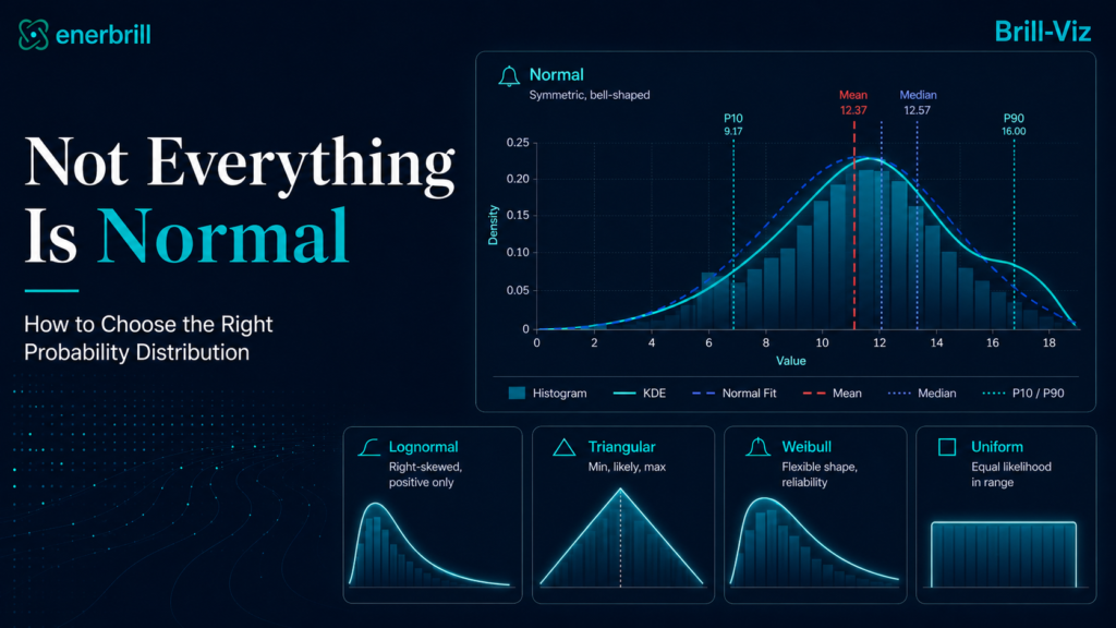
A distribution is a mathematical model of how probability is allocated across possible outcomes. It influences what appears typical, how quickly probability declines away from the center, how much remains in the tails, and whether unusual values are treated as rare or reasonably plausible.
Choosing the right probability distribution starts with checking whether the assumed model is suitable for the observed data and intended analysis. The NIST Engineering Statistics Handbook explains that distributional assumptions should be verified before they are used for statistical intervals, hypothesis tests, or simulations.
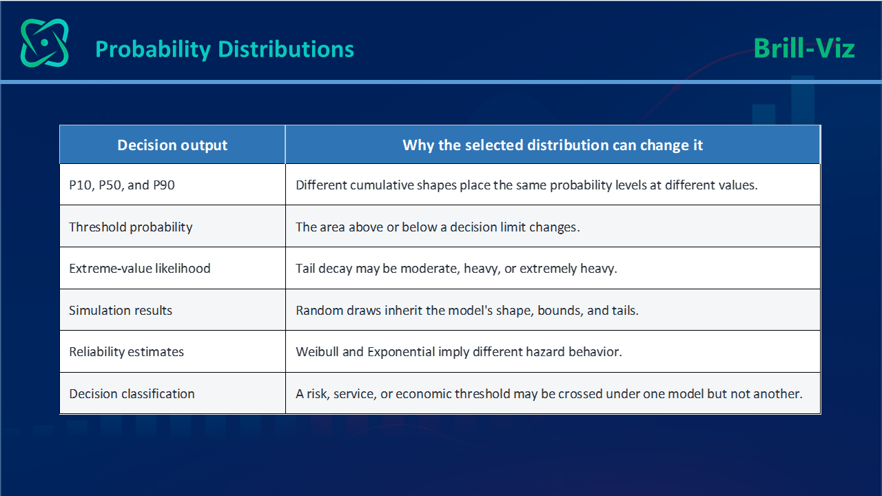
That is why distribution choice is not a cosmetic decision. It may change P10, P50, and P90, the probability of crossing a threshold, simulated extremes, reliability estimates, and the apparent level of risk.
The Most Common Distribution Mistake
Everyone knows the first mistake: assuming every dataset should be Normal. Here is the sneakier one, assuming that two curves which look almost identical near the center must behave the same way everywhere else. They often do not, and the difference shows up exactly where it matters most, i.e. the tails.
The Brill-Viz Probability Distribution Library
Both Grouped and Smart-Stats, in Brill-Viz, contain a broad and analytically meaningful set of continuous distributions:
The current library covers symmetric, skewed, bounded-range, and progressively heavy-tailed behavior. It is broad enough for a strong continuous-distribution workflow without pretending that any fixed library contains every possible model.
Visual Reference: The Distributions Available in Brill-Viz
The following figure represents the current Smart and Grouped Stats probability distributions:
Why Similar-Looking Distributions Are Not Interchangeable?
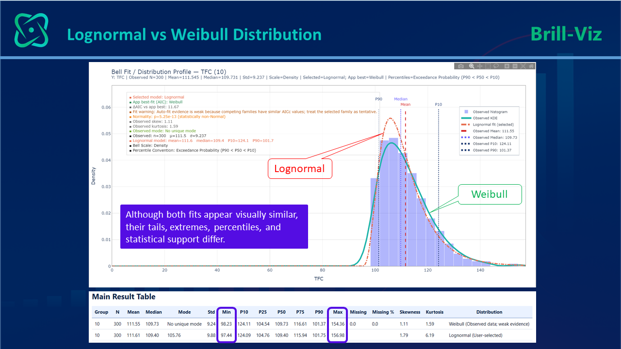
1. Positive and right-skewed: Lognormal, Gamma, Weibull, and Exponential
All four can occupy the positive axis and decline to the right, but they represent different mechanisms and can produce different upper-tail probabilities.
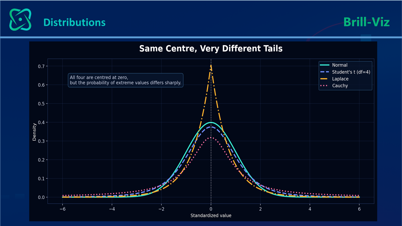
2. Symmetric but increasingly heavy-tailed: Normal, Student’s t, Laplace, and Cauchy
These distributions can all be centered at the same value, yet they differ sharply in how much probability they allocate to extreme deviations.
3. Same bounds, different assumptions: Uniform vs Triangular
Both are bounded by a minimum and maximum. Uniform treats every value in the interval as equally likely. Triangular gives more probability near a specified most-likely value. Their ranges can be identical while their percentiles and simulated central concentration differ.
A Real Modeling Choice: Auto Says Lognormal, the Analyst Selects Gamma
Suppose Auto (AIC) identifies Lognormal as the strongest candidate, but the analyst selects Gamma. The Gamma curve may still look acceptable around the main body of the histogram. That visual similarity can hide a meaningful difference in the upper tail.
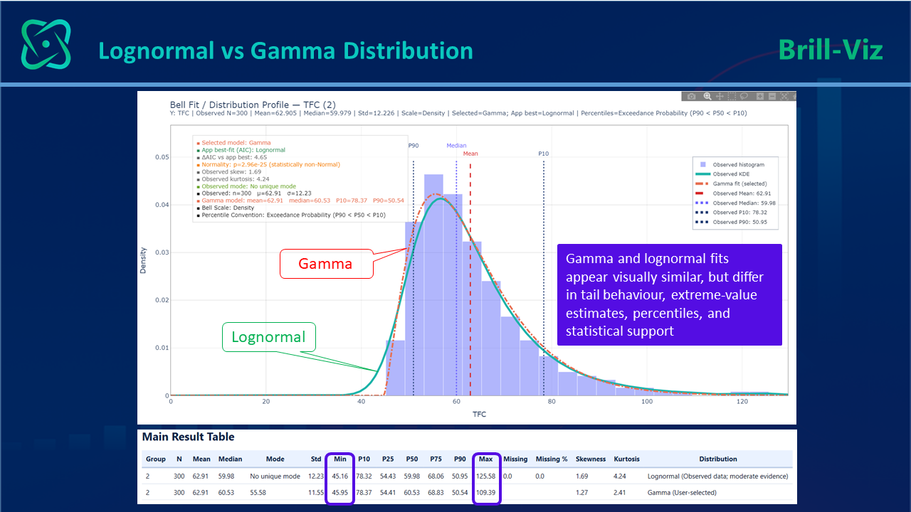
A fitted Lognormal may preserve more probability in very high values than a comparable Gamma model. Selecting Gamma could therefore reduce an upper percentile or the probability of exceeding a high threshold. The exact direction and magnitude depend on the fitted parameters, so the effect must be compared rather than assumed.
Common Overrides and Their Possible Consequences
Every override choice above ultimately serves the same goal: turning uncertainty into a measurable basis for decisions. (The distinction between uncertainty and risk is covered in the companion article, “Beyond the Average".) The remaining question is how to choose, in practice, between the automatic recommendation and a manual override.
How Automatic Fitting and Manual Selection Differ
When automatic fit and process knowledge agree, confidence increases. When they disagree, the difference should be investigated, compared, and reported.
Statistical fit should be combined with knowledge of the process being analyzed. NIST’s guidance on choosing an appropriate distribution model recommends selecting models that make practical sense, fit the data, and have a plausible theoretical justification where possible.
What “Best Fit” Actually Means
Best fit means that one candidate performs better than the other supported candidates under the selected comparison method and observed sample. AIC ranks relative fit while penalizing unnecessary complexity; lower AIC generally indicates a better balance among the candidates compared.
In practice, Auto (AIC) fits every supported distribution to the data and selects whichever one produces the lowest AIC score, i.e. the entire mechanism behind the “Auto” recommendation.
It does not mean that the distribution is permanently proven to be the true process. Results can be affected by sample size, outliers, truncation, mixtures of groups, measurement limits, missing extremes, and the candidate families included.
How Brill-Viz Turns the Theory into a Practical Workflow
Understanding the theory is one thing; applying it fast, correctly, and repeatably is another. This is exactly where Brill-Viz's Smart and Grouped Stats take over, i.e. fitting the observed distribution, running an automatic AIC comparison, allowing manual overrides, layering grouped comparisons, and generating percentiles, interpretations, and publication-ready outputs in one pass.
Before Overriding Auto-Fit: Seven Questions
Common Mistakes
Key Takeaways
Closing Remarks
A probability distribution is not decorative mathematics. It is a model of where outcomes concentrate, how far they can spread, and how much probability remains in the tails. Those properties directly influence what appears likely, conservative, optimistic, safe, or risky.
Brill-Viz Grouped Stats already provides a strong and coherent distribution library. Its value lies not in offering every distribution ever developed, but in combining a meaningful candidate set with automatic AIC comparison, user-controlled alternatives, grouped analysis, and transparent reporting.
The best practice is neither blind automation nor unrestricted manual choice. It is a disciplined combination: let the data speak, let domain knowledge challenge or confirm it, compare the consequences, and report the decision honestly.
Why similar-looking curves can produce different probabilities, and how evidence and judgment should work together?
The observations may remain the same, but the probability story changes when a different distribution is fitted, which can alter percentiles, tail probabilities, simulations, reliability conclusions, and decisions.
Choosing the right probability distribution is essential because similar-looking models can produce very different estimates of uncertainty, tail risk, and extreme outcomes.
Before you start: This article builds on the companion piece, “Beyond the Average: What the Bell Curve Reveals About Risk and Uncertainty.” If you haven’t read it yet, start there for the basics on distributions, spread, and the difference between uncertainty and risk.
TL;DR
A probability distribution is not just a curve someone drew over your histogram, it is the model deciding how probability gets allocated around the center, through the shoulders, and out into the tails. Pick the wrong one, and the tails will lie to you. Brill-Viz Grouped Stats currently supports Auto (AIC, the Akaike Information Criterion), Normal, Lognormal, Gamma, Weibull, Student’s t, Exponential, Uniform, Triangular, Laplace, and Cauchy. Together, these distributions already provide a powerful continuous-distribution library covering symmetric, skewed, waiting-time, reliability, bounded-range, and progressively heavy-tailed behavior. A defensible choice combines statistical fit, process meaning, tail behavior, and transparent comparison whenever a user overrides the automatic recommendation.
Why Distribution Choice Matters
A distribution is a mathematical model of how probability is allocated across possible outcomes. It influences what appears typical, how quickly probability declines away from the center, how much remains in the tails, and whether unusual values are treated as rare or reasonably plausible.
Choosing the right probability distribution starts with checking whether the assumed model is suitable for the observed data and intended analysis. The NIST Engineering Statistics Handbook explains that distributional assumptions should be verified before they are used for statistical intervals, hypothesis tests, or simulations.
That is why distribution choice is not a cosmetic decision. It may change P10, P50, and P90, the probability of crossing a threshold, simulated extremes, reliability estimates, and the apparent level of risk.
Core distinction
The data are the observations. The fitted distribution is the model placed over those observations. Changing the model does not change the historical data, but it can change what we infer about unobserved and future outcomes.
The Most Common Distribution Mistake
Everyone knows the first mistake: assuming every dataset should be Normal. Here is the sneakier one, assuming that two curves which look almost identical near the center must behave the same way everywhere else. They often do not, and the difference shows up exactly where it matters most, i.e. the tails.
- Positive variables such as permeability, income, field size, or revenue may be strongly right-skewed.
- Failure and lifetime data may require a hazard-based Weibull model rather than a generic positive distribution.
- Waiting time at a constant event rate may be closer to Exponential.
- Expert ranges based on minimum, most-likely, and maximum values may be represented by Triangular rather than a fitted historical distribution.
- Symmetric data may still have much heavier tails than Normal, making Student’s t, Laplace, or Cauchy materially different.
- Two distributions can fit the center similarly while assigning very different probability to the tails.
The Brill-Viz Probability Distribution Library
Both Grouped and Smart-Stats, in Brill-Viz, contain a broad and analytically meaningful set of continuous distributions:
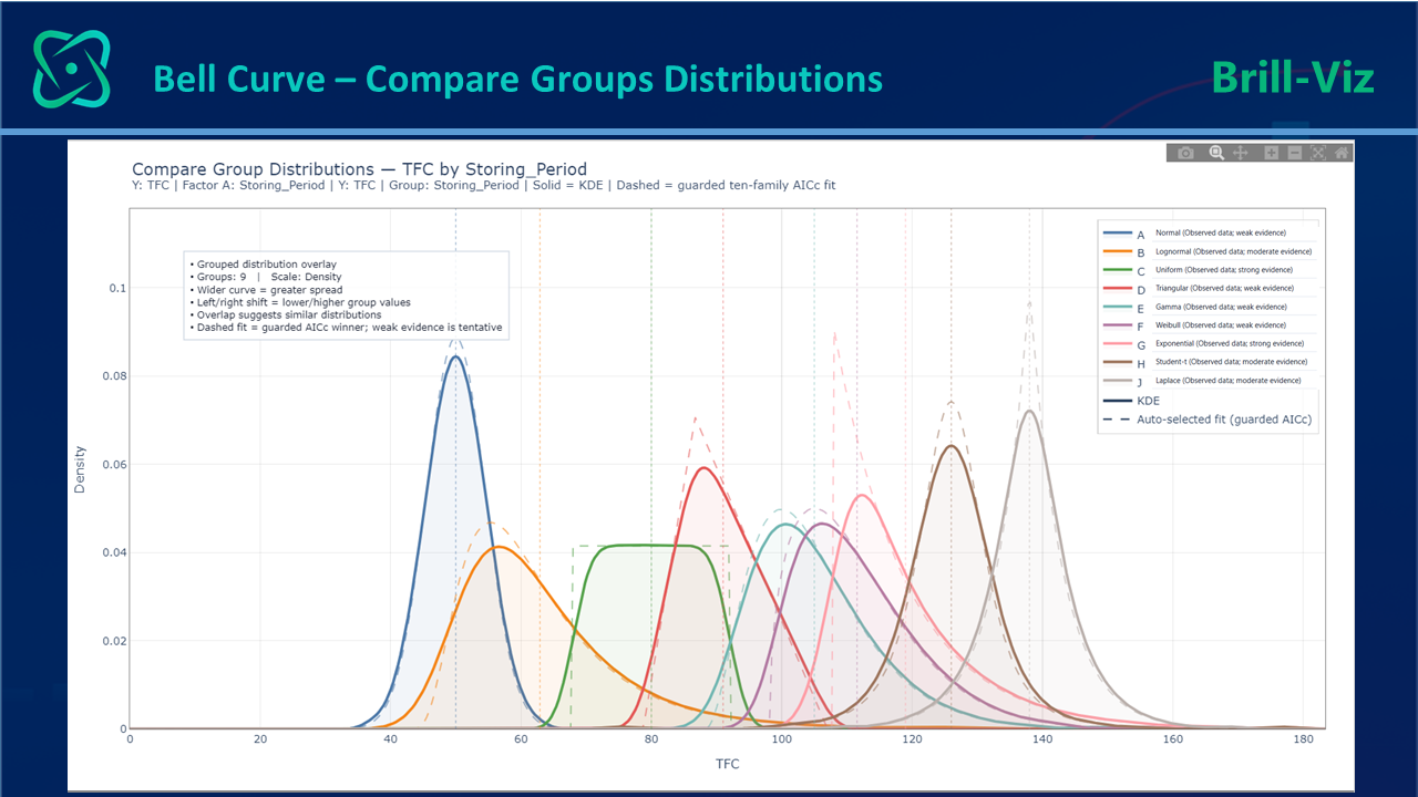
Figure 1. The Brill-Viz continuous-distribution library at a glance: Normal, Lognormal, Gamma, Weibull, Student’s t, Exponential, Uniform, Triangular, Laplace, and Cauchy.
The current library covers symmetric, skewed, bounded-range, and progressively heavy-tailed behavior. It is broad enough for a strong continuous-distribution workflow without pretending that any fixed library contains every possible model.
This library is already sufficient for a strong continuous-distribution workflow. Future additions may extend specialized use cases, but their absence does not weaken the current core capability.
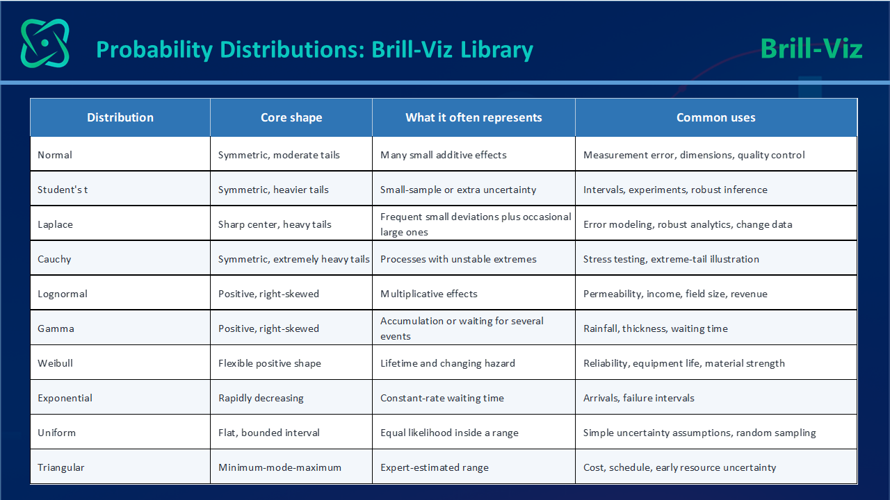
Visual Reference: The Distributions Available in Brill-Viz
The following figure represents the current Smart and Grouped Stats probability distributions:
Figure 2. Each Brill-Viz-supported distribution plotted individually: Normal, Lognormal, Gamma, Weibull, Student’s t, Exponential, Uniform, Triangular, Laplace, and Cauchy
Why Similar-Looking Distributions Are Not Interchangeable?
1. Positive and right-skewed: Lognormal, Gamma, Weibull, and Exponential
All four can occupy the positive axis and decline to the right, but they represent different mechanisms and can produce different upper-tail probabilities.
- Lognormal commonly reflects multiplicative effects and can retain substantial probability in the upper tail.
- Gamma often represents accumulation or waiting until several positive contributions occur.
- Weibull is driven by its shape parameter and can represent decreasing, constant, or increasing hazard.
- Exponential is the constant-hazard special case and has a comparatively simple rapidly declining tail.
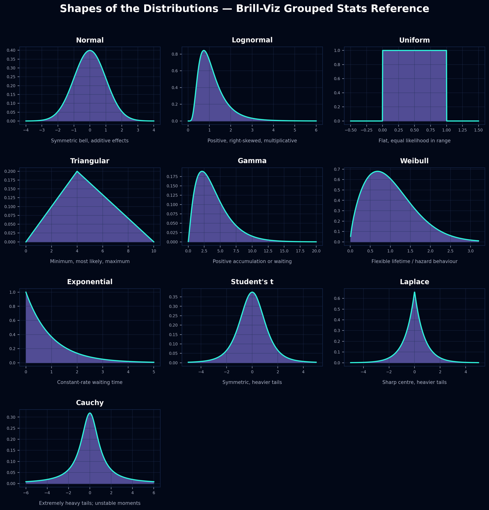
Figure 3. Comparison of lognormal and Weibull fits, illustrating differences in distribution shape, tails, percentiles, and summary statistics.
2. Symmetric but increasingly heavy-tailed: Normal, Student’s t, Laplace, and Cauchy
These distributions can all be centered at the same value, yet they differ sharply in how much probability they allocate to extreme deviations.
Figure 4. The same center does not imply the same tail risk. Student’s t and Laplace are heavier-tailed than Normal; Cauchy is more extreme and does not have a finite theoretical mean or variance.
Normal vs Student’s t
Both are smooth and symmetric. Student’s t assigns more probability to the tails, especially with low degrees of freedom (roughly, how much data the estimate is based on , fewer observations means lower degrees of freedom and heavier tails). Choosing Normal when Student’s t is more appropriate may create intervals that are too narrow and make unusual outcomes appear less likely.
Student’s t vs Cauchy
Cauchy is a special Student’s t case with one degree of freedom. Its tails are so heavy that a theoretical mean and variance do not exist. Selecting Cauchy is a major modeling decision: sample averages may remain unstable, and standard deviation-based interpretation becomes unreliable.
Normal vs Laplace
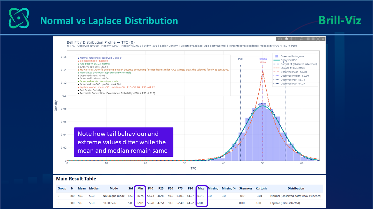
Laplace has a sharper peak and heavier tails than Normal. It places more probability very near the center and in the extremes, with less in the intermediate shoulders. A Normal fit can therefore smooth away both central concentration and tail exposure.
Figure 5. Normal and Laplace distributions with similar central values but different tail behavior and extremes
Why this matters
Using Normal for genuinely heavy-tailed data can make intervals too narrow and extreme outcomes appear less likely than the model evidence supports.
3. Same bounds, different assumptions: Uniform vs Triangular
Both are bounded by a minimum and maximum. Uniform treats every value in the interval as equally likely. Triangular gives more probability near a specified most-likely value. Their ranges can be identical while their percentiles and simulated central concentration differ.
A Real Modeling Choice: Auto Says Lognormal, the Analyst Selects Gamma
Suppose Auto (AIC) identifies Lognormal as the strongest candidate, but the analyst selects Gamma. The Gamma curve may still look acceptable around the main body of the histogram. That visual similarity can hide a meaningful difference in the upper tail.
Figure 6. Comparison of gamma and lognormal fits showing similar central behavior but differences in tails, extremes, percentiles, and model support
A fitted Lognormal may preserve more probability in very high values than a comparable Gamma model. Selecting Gamma could therefore reduce an upper percentile or the probability of exceeding a high threshold. The exact direction and magnitude depend on the fitted parameters, so the effect must be compared rather than assumed.
Manual selection is not automatically wrong
It becomes defensible when a process-based reason, industry assumption, or scenario objective is stated and its consequences are shown.
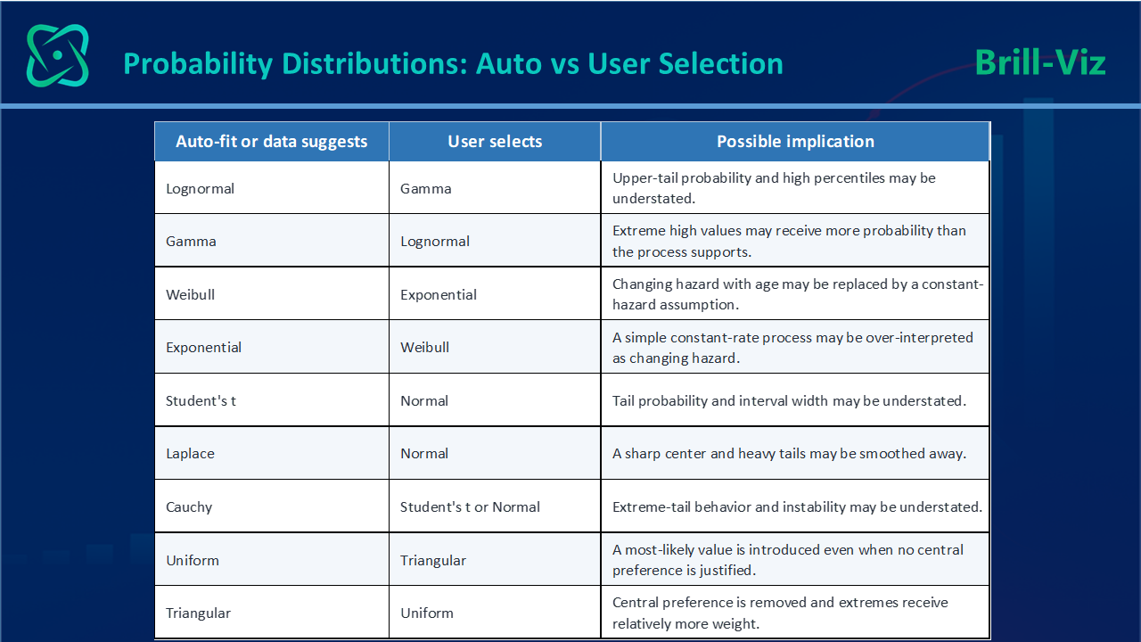
Common Overrides and Their Possible Consequences
These are possible, not guaranteed, effects. Parameters, sample size, truncation, and decision thresholds determine the actual difference.
Every override choice above ultimately serves the same goal: turning uncertainty into a measurable basis for decisions. (The distinction between uncertainty and risk is covered in the companion article, “Beyond the Average”.) The remaining question is how to choose, in practice, between the automatic recommendation and a manual override.
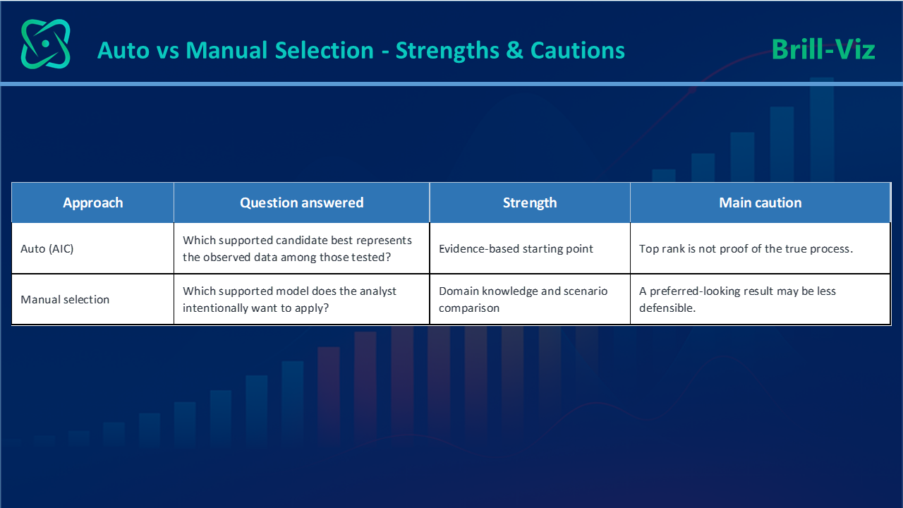
How Automatic Fitting and Manual Selection Differ
When automatic fit and process knowledge agree, confidence increases. When they disagree, the difference should be investigated, compared, and reported.
Statistical fit should be combined with knowledge of the process being analyzed. NIST’s guidance on choosing an appropriate distribution model recommends selecting models that make practical sense, fit the data, and have a plausible theoretical justification where possible.
What “Best Fit” Actually Means
Best fit means that one candidate performs better than the other supported candidates under the selected comparison method and observed sample. AIC ranks relative fit while penalizing unnecessary complexity; lower AIC generally indicates a better balance among the candidates compared.
In practice, Auto (AIC) fits every supported distribution to the data and selects whichever one produces the lowest AIC score, i.e. the entire mechanism behind the “Auto” recommendation.
It does not mean that the distribution is permanently proven to be the true process. Results can be affected by sample size, outliers, truncation, mixtures of groups, measurement limits, missing extremes, and the candidate families included.
How Brill-Viz Turns the Theory into a Practical Workflow
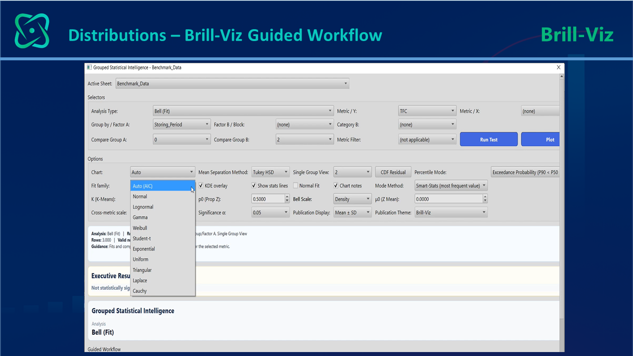
Understanding the theory is one thing; applying it fast, correctly, and repeatably is another. This is exactly where Brill-Viz’s Smart and Grouped Stats take over, i.e. fitting the observed distribution, running an automatic AIC comparison, allowing manual overrides, layering grouped comparisons, and generating percentiles, interpretations, and publication-ready outputs in one pass.
Figure 7. The workflow showing the Auto (AIC) recommendation with manual override dropdown.
Step 1: Start with Auto (AIC – Akaike Information Critrion)
Use the automatic result as an evidence-based starting point. Review the best-fit name, histogram, KDE, fitted curve, AIC information, normality result, skewness, and percentile range.
Step 2: Select manually only for a defensible reason
Manual selection can support domain knowledge, an industry convention, controlled scenario analysis, or a known process assumption. It should not be used merely because a distribution is familiar or produces preferred percentiles.
Step 3: Compare the override
- Compare fit measures where available.
- Inspect the center, shoulders, and both tails.
- Compare P10, P50, P90, mean, median, and spread.
- Compare probabilities above and below decision thresholds.
- For reliability analysis, compare Weibull and Exponential hazard implications.
- For heavy-tailed data, compare Normal, Student’s t, Laplace, and Cauchy carefully.
- For grouped analysis, check whether one forced distribution masks genuine differences.
Step 4: Report transparently
A strong report distinguishes the application-recommended best fit from the user-selected model. Where they differ, state the reason and show how the choice changes decision-relevant outputs.
Recommended reporting language
“Auto (AIC) identified Lognormal as the strongest candidate. Gamma was selected manually for scenario comparison. The Gamma assumption produced a lower upper percentile and a smaller probability of exceeding the operational threshold. The result is therefore model-dependent”.
Before Overriding Auto-Fit: Seven Questions
- What process-based reason supports the alternative distribution?
- Does its support and shape make sense for the variable?
- How much weaker is its fit relative to the automatic recommendation?
- How does it change P10, P50, P90, spread, and tail probabilities?
- Does it change the probability of crossing a decision threshold?
- Am I choosing it because it is defensible or because I prefer its result?
- Will the report clearly identify it as a user-selected assumption?
Common Mistakes
- Assuming Normality without testing it.
- Treating the lowest AIC as unquestionable proof.
- Choosing a curve by its center while ignoring the tails.
- Overriding Auto (AIC) without comparing percentiles and threshold probabilities.
- Using Cauchy without recognizing that its theoretical mean and variance are undefined.
- Treating Exponential and Weibull as interchangeable despite different hazard assumptions.
- Forcing one distribution across groups that behave differently.
- Reporting a manually selected fit without documenting the assumption.
Key Takeaways
- Not everything is Normal, and similar-looking distributions are not interchangeable.
- The current Grouped Stats library is already broad and powerful for continuous distribution analysis.
- Auto (AIC) is an evidence-based recommendation; manual selection is an explicit modeling assumption.
- Changing the distribution can change percentiles, tail probabilities, simulations, reliability estimates, and decisions.
- Normal, Student’s t, Laplace, and Cauchy provide a valuable progression from moderate to extreme tail behavior.
- Lognormal, Gamma, Weibull, and Exponential cover different positive and right-skewed processes.
- Uniform and Triangular represent different assumptions even when they share the same minimum and maximum.
- When users override auto-fit, they should compare and report the consequences.
Closing Remarks
A probability distribution is not decorative mathematics. It is a model of where outcomes concentrate, how far they can spread, and how much probability remains in the tails. Those properties directly influence what appears likely, conservative, optimistic, safe, or risky.
Brill-Viz Grouped Stats already provides a strong and coherent distribution library. Its value lies not in offering every distribution ever developed, but in combining a meaningful candidate set with automatic AIC comparison, user-controlled alternatives, grouped analysis, and transparent reporting.
The best practice is neither blind automation nor unrestricted manual choice. It is a disciplined combination: let the data speak, let domain knowledge challenge or confirm it, compare the consequences, and report the decision honestly.
Related reading: If you haven’t already, start with the companion article, “Beyond the Average: What the Bell Curve Reveals About Risk and Uncertainty”. It covers why the average alone is not enough, what a bell curve shows, and how uncertainty and risk relate to one another; the foundation this article is built on.
Q: Are the distributions currently available in Grouped Stats sufficient?
Answer: Yes. They already cover the principal continuous shapes needed for symmetric, skewed, waiting-time, reliability, bounded-range, and heavy-tail analysis. Future additions may broaden specialised use cases, but they are not required for a powerful core workflow.
Q: Does Auto (AIC) mean the selected distribution is certainly true?
Answer: No. It identifies the strongest candidate among the supported models tested under the available sample and criteria.
Q: Why include both Laplace and Cauchy?
Answer: They expose heavy-tail behavior that Normal can miss. Laplace combines a sharp center with heavy tails; Cauchy represents a much more extreme case and requires special caution.
Q: Can two distributions look almost identical but produce different decisions?
Answer: Yes. Small visual differences in the tails can produce meaningful differences in upper percentiles, threshold probabilities, and simulated extremes.
Q: If Lognormal is best fit, is selecting Gamma always wrong?
Answer: Gamma may be defensible for a process or scenario reason, but its fit and consequences should be compared and documented.
Q: Should every group use the same distribution?
Answer: Not necessarily. Different groups may have different mechanisms, skewness, and tail behavior. Grouped analysis is valuable because a combined fit can hide those differences.
Answer: Yes. They already cover the principal continuous shapes needed for symmetric, skewed, waiting-time, reliability, bounded-range, and heavy-tail analysis. Future additions may broaden specialised use cases, but they are not required for a powerful core workflow.
Answer: No. It identifies the strongest candidate among the supported models tested under the available sample and criteria.
Answer: They expose heavy-tail behavior that Normal can miss. Laplace combines a sharp center with heavy tails; Cauchy represents a much more extreme case and requires special caution.
Answer: Yes. Small visual differences in the tails can produce meaningful differences in upper percentiles, threshold probabilities, and simulated extremes.
Answer: Gamma may be defensible for a process or scenario reason, but its fit and consequences should be compared and documented.
Answer: Not necessarily. Different groups may have different mechanisms, skewness, and tail behavior. Grouped analysis is valuable because a combined fit can hide those differences.